

This project was completed before I did the bulk of my ML coursework and research in college and before I had become fully familiarized with Python. Accordingly, you'll find some quirky naming conventions, a GitHub Repo that isn't exactly organized, some non-standard metrics, and a very trial-and-error-oriented approach to designing the models. We all start somewhere :)
Overview
Songs with vocals can often be broken into different parts, such as verses, choruses, bridges, etc. Such a segmentation task is easy if there are song lyrics that annotate the different parts of the song in those categories. But in the absence of such lyrics, determining which type of song segment is playing based purely on how it sounds is more challenging.
With practice, humans can become reasonably accurate at this task – I did, out of necessity for a volunteering role I held in high school. Can a computer do the same? Let's figure it out together!
Take a look at the Github repo below to see the code I wrote for this project – I'll be referencing it throughout this post. Shoutout to my church family at home – I love hanging out and serving alongside you all! Special thanks goes to MIT's 6.036 Introduction to Machine Learning course for teaching me the fundamentals of machine learning last semester and reigniting my excitement about this subfield of computer science!
 tothepowerofn
Motivation: Replaced by a Machine
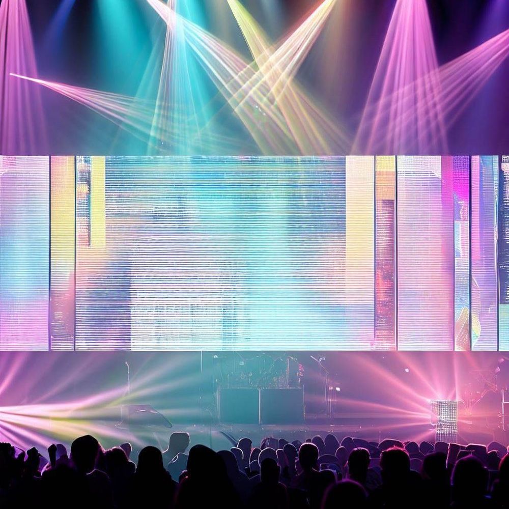
To those of you who have never attended a Protestant church service in the southern United States, the phrase "church service" may evoke images of aged parishioners singing hymns and praying quietly on a Sunday morning. Yet in the South, that phrase takes on a new meaning in the many churches equipped with auditoriums that look like more like concert halls than chapels.
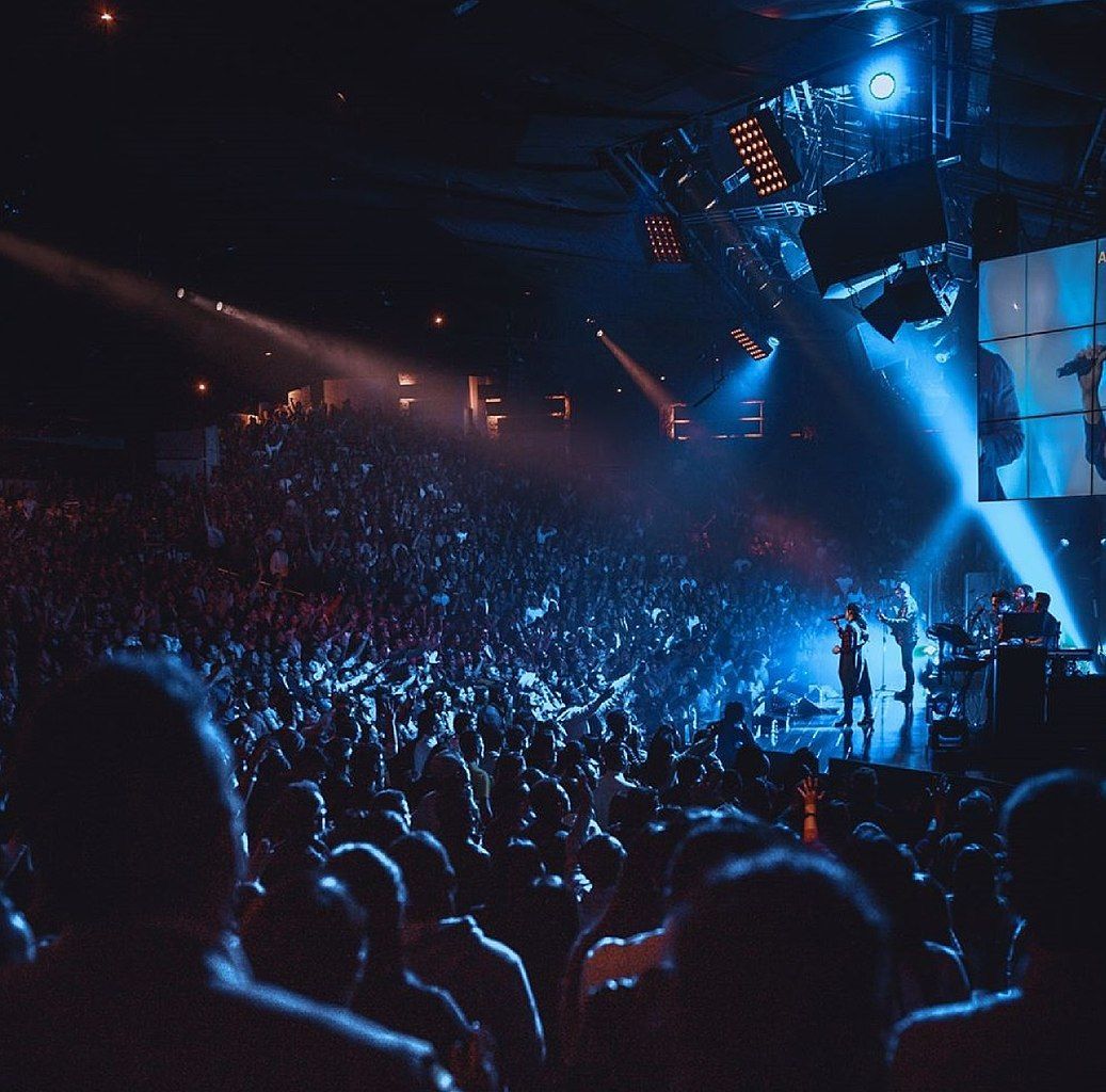
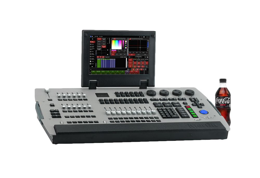
During high school, my favorite way to spend free time was to volunteer at my church to run the lighting console during services. I loved working with my other friends who served, and I enjoyed programming and the lighting console that controlled dozens of colored, movable fixtures around the stage.
During worship, I was tasked with running different routines (which are called cues) during different parts of the songs. I always prided myself on being able to execute these cues at the optimal times during the music such that the lighting changes on stage matched the sound of the music at that moment.
Even since I started college in Boston, I still enjoy doing the lights whenever I can during visits back home. So you can imagine my shock when, one day, my mentor from church (we will call them M) delivered some painful news.In other words: my job had been taken by a simple trigger that changed the lights based on the lyrics slides on the screen! I decided to text a group chat with M and some of my other friends from church, only to be roasted:
Hi,
I wanted to share a new change we have made to how we are doing lighting at our campuses.
When we opened our new campus we simplified on how we are running lights. We found out that going to a more simplified system of running lights was a big win and we had more engagement. With that said we are going to be moving to this model of running lights. Below is how we are going to be running lights moving forward.
Pro Presenter will fire the lighting cue for each part of service and songs. Starting in November we will not need a lighting operator for most weekend services. Let me encourage you to continue to serve with us in other areas such as Pro Presenter or Director or even some opportunities during our midweek services. Love you all! Thank you for journeying this out with us!
Thanks, M.
In other words: my job had been taken by a simple trigger that changed the lights based on the lyrics slides on the screen! I decided to text a group chat with M and some of my other friends from church, only to be roasted:
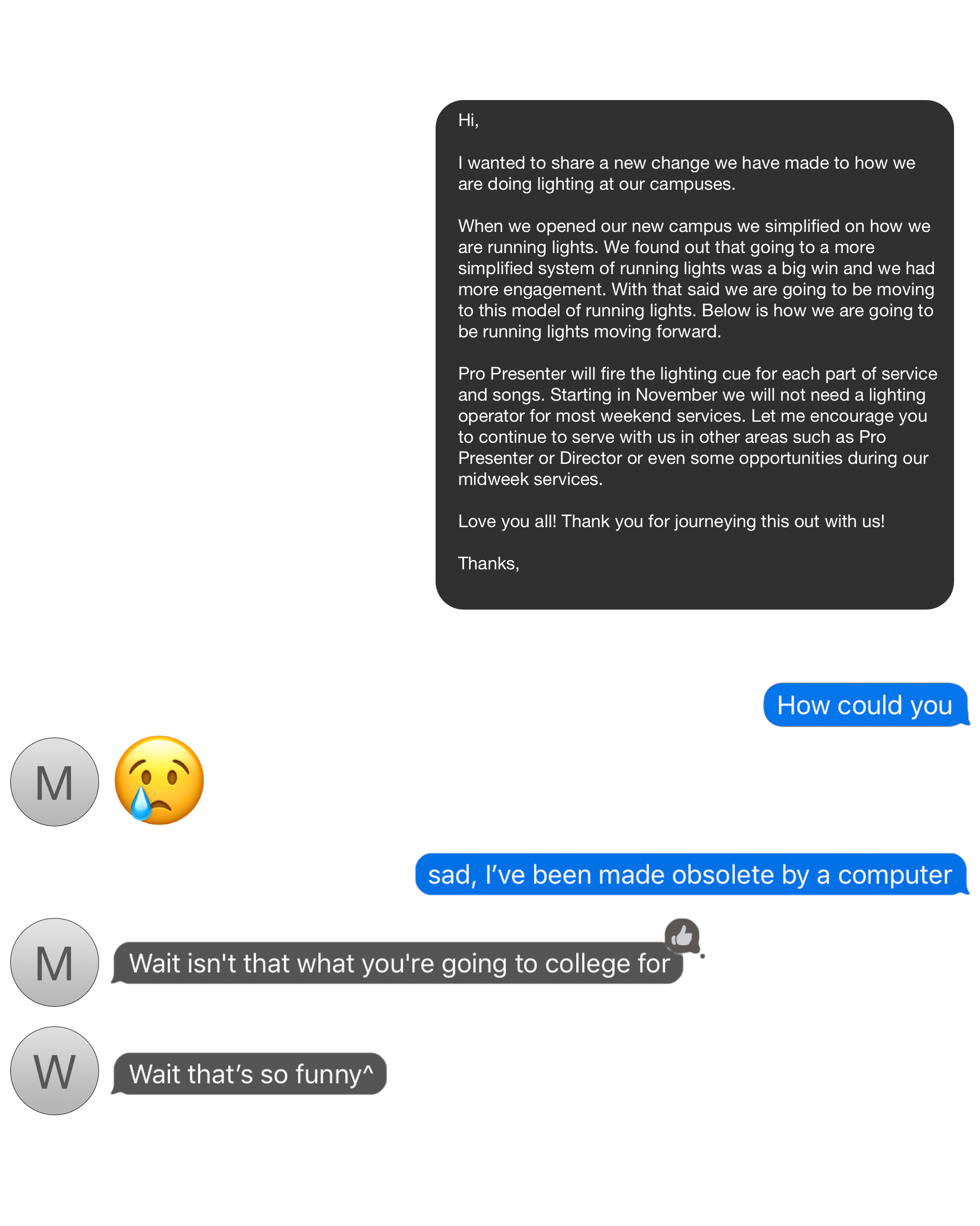
M is right – this is the sort of thing that I am in college for. But, while I’ve always been a friend of machines and a supporter of their eventual takeover, to be replaced by such a simple form automation hurt! The trigger was thoughtless. It was connected to the song lyrics on the screen, and fired mechanically based upon slide number – without feeling the music! Moreover, it was needy – the triggers would need to be tediously set up for each song in advance (i.e. advance to cue chorus when slide 9 appears). I was eager to design a better solution!
Specifying the Problem

Goal
The goal is to design an automated system that will be reasonably accurate in tagging parts of a song with the appropriate song segment type (verse, chorus, etc.). At a given point in the song, the automated solution should make decisions onlyon current and previous information in the song. This emulates the task I face while running the light console– at a given moment, I am tasked with choosing a song cue based only on what I am hearing at the moment and what I have heard previously.
As we will discuss later, this automated task is actually harder than my task when running the lights. Why? Because during service, I have usually heard the entire song before (during rehearsal) and have received feedback by the service Director or Producer. In contrast, our automated solution will be tagging a song in real time (from its perspective), never having heard the song before.
Song Segment Types
We now turn our attention to types of song segments:
Intro: The song is just beginning. The first verse has not begun. The singer(s) may be making some initial remarks, or the band may be playing in the absence of any vocals.
Verse: " ... a unit that prolongs the tonic....the musical structure of the verse nearly always recurs at least once with a different set of lyrics ... " - Wikipedia
Chorus: "the element of the song that repeats at least once both musically and lyrically. It is always of greater musical and emotional intensity than the verse." - Wikipedia
Instrumental: No words on the lyrics sheet are being sung: the singer(s) may be silent; the singer(s) may be singing non-lexical vocables; the singer(s) may be talking.
Bridge: " ... a section of a song with a significantly different melody ..." - Wikipedia
End: The song is ending: the singer(s) may be silent; the singer(s) may be making some final remarks; the singer(s) may be singing non-lexical vocables.
Note that when generating training data (which came from recordings or worship on my church's YouTube channel), I chose to tag song parts based on my musical intuition loosely guided by official lyric sheets, allowing the former to overrule the latter in cases of conflict. For instance, there were a couple songs in which a previous verse was sung over a melody that seemed bridge-like, leading me to tag that portion as bridge. Why did I do this? Because I wanted a model that learns to tag based on melody, not on lyrics (this is not a speech recognition task over sung words).
Furthermore, the tags above do not encompass all possible music segment types, so some segment types were merged into others. For example, I chose to merge pre-choruses into verses, and tags (the musical kind) into bridges. This was for simplicity. Perhaps a future project will include more segment tag types!
Describing the Problem Intuitively
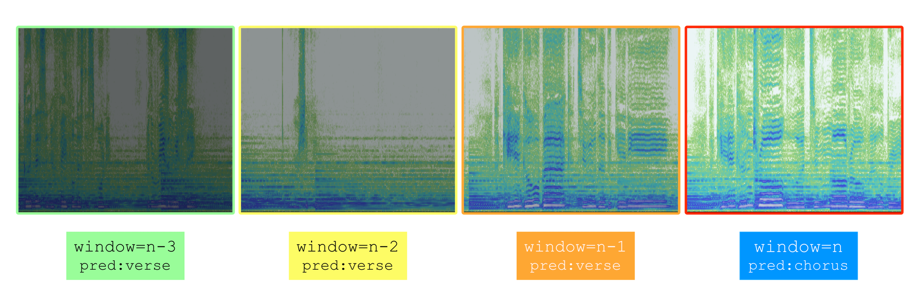
The first step to solving this problem is to enter my perspective while running the lighting console. I consider the song a sequence. Every few seconds, I think about how the song has sounded in that window of a few seconds, and about how I remember it sounding in the seconds prior to that window. Then, I decide what song segment type is currently playing. Based on that decision, I either advance to a new cue (if the song segment type that I think was just playing does not match the cue name active on the console) or remain on the cue currently being executed (if the song segment type I think was just playing does match the cue on the console). Thus, the song can be considered a sequence of small windows/snippets of audio pieced together, with each window being predicted as a particular song segment type.
With this intuition, it becomes clear how to represent this task as a supervised sequence-to-sequence machine learning classification problem:
Given a sequence of consecutive windows of audio, the model should output a sequence of song segment types corresponding to each window. For a given window of audio, the model must decide, using only information from this current window and information from previous windows of audio, what type of song segment type is being played. The model will be able to learn from examples, where an example is a sequence of audio windows that have each been labeled with song segment type (by me).
Now, the description above is a bit vague – "windows of audio" is technically imprecise. Instead, we must decide how to represent each window of audio with some set of features (more on that later) so that the model can understand it.
Audio Representation
Representing audio on a computer is baffling if you have never thought about it before. There are many different formatsin which audio may be stored on a computer, but ultimately all of these representations are stored as 0's and 1's in computer memory.
For many machine learning applications, audio data is first represented with uncompressed WAV files. These WAV files store a large sequence of numbers representing a PCM stream that describes the analog signal of the audio. This sequence contains numbers that correspond to samples of the audio waveform at periodic intervals.
To understand how large these sequences of numbers are, consider a simple 5 second clip of audio stored as an uncompressed, unsigned 16-bit integer WAV file at a sampling rate of 22,050 samples per second. That means that for each second, the WAV file contains 22,050 integers. For our 5 second audio clip, that means we'll be storing 110,250 integers!
To a human, it may seem like a lot of information for a 5-second audio clip, but computers are quite good at quickly reading these numbers and producing the corresponding audio through speakers in real time (22,050 integers per second for 1 second of audio). But what about when the computer has to do more than simply translate these many numbers into noises? What if the computer has to think about all of those numbers and make decisions about them? Things become much more complicated – in fact, unmanageable for machine learning problems on today's computers.
This motivates finding some other representation for our audio that is much more compact than a WAV file. We need to find a way to represent chunks of audio in way fewer numbers than a WAV file does. In doing so, we will inherently lose information (2000 integers will certainly store less information than 22,050 integers). But it turns out that our machine learning model doesn't need much of that information to make good decisions – it can decide the type of song segment playing for a given second of audio based on much less than 22,050 integers.
Featurizing the Audio
What are Features, and Why do We Need Them?
This brings us to featurizing the audio. As Wikipedia states, "a feature is an individual measurable property or characteristic of a phenomenon being observed." To better understand what a feature is, consider the case where you are attempting to predict if, on a given day, I ate cake for lunch. A feature might be the number of calories I ate during lunch. Another might be my blood sugar levels shortly after the meal. Yet another could be the number of calories in the entree for that day.
For supervised learning problems, choosing good features helps your model train quickly and efficiently to make good predictions. If I tasked you with predicting if I ate cake on a given day for lunch and gave you the choice of watching the day's cafeteria video security footage (which can be considered a feature that describes the changing of pixels on the CCTV screen through 24 hours) or receiving the 3 features mentioned in the previous paragraph, you would probably pick the latter. Why? It's quicker, as there's less information to process (you don't have to sit and watch a long video and pick me and my tray out in a sea of people), and you can probably make pretty good predictions with those 3 features I gave you.
The same is true for our machine learning model and audio. Feeding it raw waveform audio data would be overwhelming, unnecessary, and would probably slow our training process to a crawl. Instead, we need to pick out features that succinctly describe the audio without overpowering the model with information.
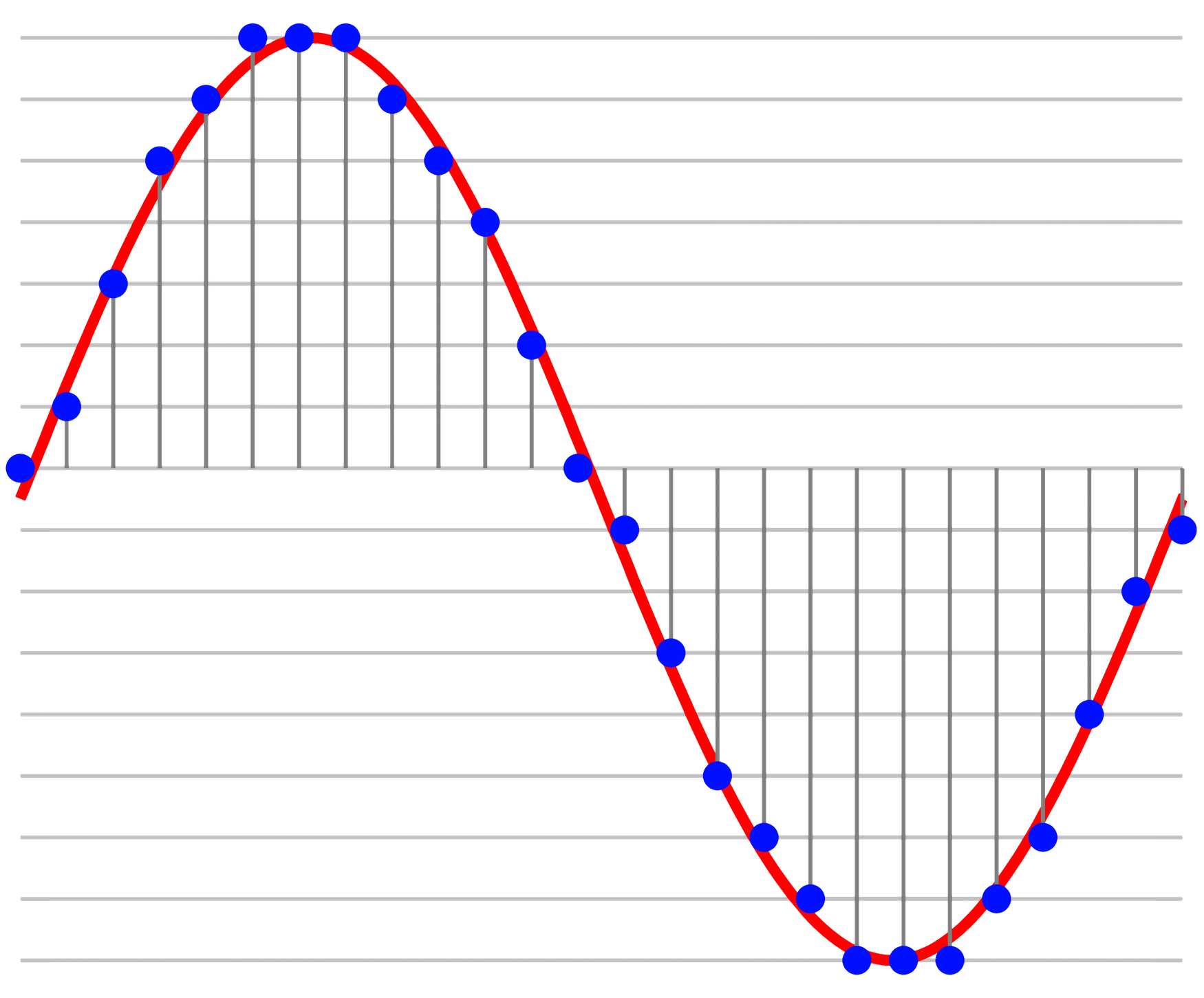
MFCC Features
It turns out for many machine learning audio tasks, MFCC features do just that for a small chunk of sound. A full explanation of these features is beyond the scope of this post, but essentially, MFCC features are several numbers that describe the spectrogram of a chunk of audio (usually a few milliseconds).
Featurizing the Data with MFCC
Now, given an audio file, we want to extract MFCC features for sequential chunks in of an audio file. Librosa for Python makes that easy!
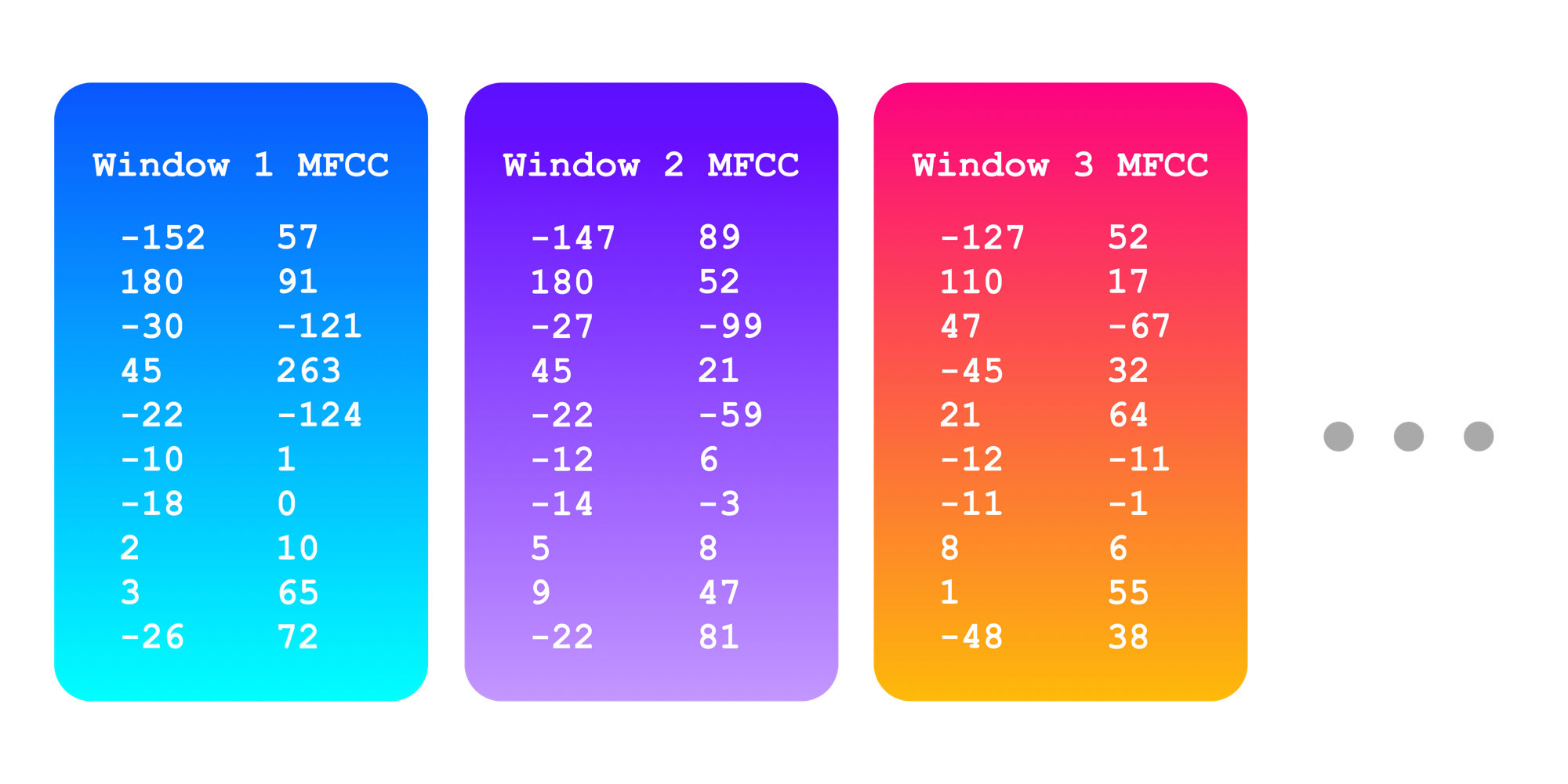
The code above extracts 20 MFCC features every 4096 waveform samples of the audio "We_Praise_You.wav," and the extraction takes place on a chunk of size 8192 samples. In this case, that means that each chunk will contain half of the next chunk (because chunk n spans 8192 samples, but chunk n+1 begins just 4096 samples ahead, leaving an overlap of 4096 samples between the two chunks).
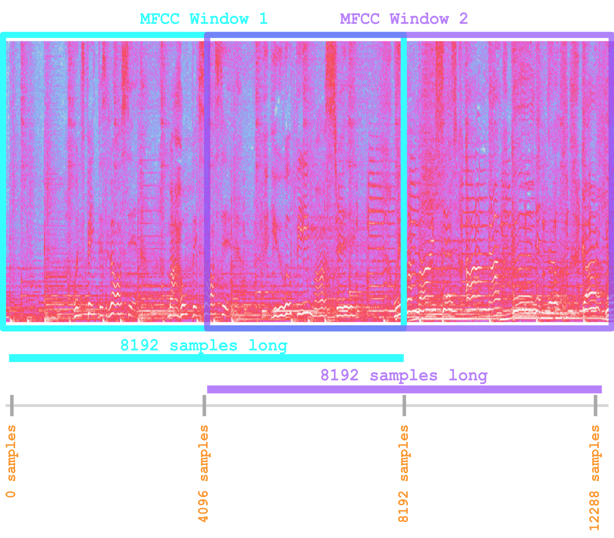
So for each MFCC chunk of 8192 samples, we get 20 numbers that describe that chunk of the audio spectrogram. We extract these overlapping windows from sample 0 and onwards in multiples of 4096 until the end of the audio.
Suppose that we have a 225 second audio clip at a sample rate of 22,050, and we're extracting 20 MFCC features for each 8192 sample chunk every 4096 samples. Then we've got 22050*225 total samples, and chunks every 4096 samples. This means we'll get (22050*225)/4096, which is approximately a sequence of 1212 sets of 20 MFCC features (when rounded up).
In this way, we can featurize each of our audio files by turning them into a sequence of MFCC features.
If you're following along in the code I wrote, you can perform MFCC extraction using code like this:
#Saves properties of the MFCC features for each song (such as length)

mfccDimIndexerModule = MFCCDimensionsIndexerModule(hop_length, n_mfcc)
indexerModulesList = [mfccDimIndexerModule]
indexer = Indexer("wavs", indexerModulesList)


# MFCCFeature will save extracted features from songs in "wav" to
# folder "mfcc_input_1".

mfccFeature = MFCCFeature("mfcc_input_1","wavs",hop_length=hop_length, n_fft=n_fft,n_mfcc=n_mfcc)
featureList = []
featureList.append(mfccFeature)


#AnnotatedSongLabeler outputs labels from segmentation guides in
#"annotations" folder. Labels will be saved to "features/labels"

annot = AnnotatedSongLabeler("annotations", sample_rate=22050, hop_length=hop_length)


#Actually extract the features to "features"

saveTrainingData("features", featureList, indexer, annot)
This code will both extract MFCC features and export labels for each MFCC window in the sequence for every song in the "wav" folder.
First, MFCC features will be extracted from the audio files in the "wav" folder in the working directory with window sizes of n_fft and hop lengths (distance between each window start) of hop_length. These MFCC features will be extracted as CSV files in the folder "features/mfcc_input_1." Each song will have a CSV file, where each row has n_mfcc columns, i.e. each row i is a window of MFCC features for the audio samples i*hop_length to i*hop_length+n_fft.
Second, for each song, the code will read in the song's annotations files in the folder "annotations" and export labels for that song in "features/labels." Each annotation CSV is a two-column spreadsheet. For each entry (row), the first column is time in seconds, and the second column specifies the song segment type (0=Intro, 1=Verse, 2=Chorus, 3=Instrumental, 4=Bridge, 5=End) that was playing up until the time in the first column. Concretely, an annotation file for a song might look like:
annotations/song-annotations.csv
| 15 | 0 |
|---|---|
| 45 | 1 |
| 60 | 2 |
| 75 | 4 |
| 90 | 2 |
| 115 | 5 |
In this example, the intro was playing for the first 15 seconds in the song, a verse was playing between seconds 15-45 of the song, a chorus was playing between seconds 45-60 of the song, a bridge was playing for seconds 60-75 of the song, another chorus was playing between 75-90 seconds of the song, and the song began was playing the ending from seconds 90-115.
The code will transform this annotations file into a labels file "features/labels/song-labels.csv." This CSV will have the same number of rows as the MFCC features CSV, and will label each row with the actual song segment type according to the segments specified in the annotations file.
Model Training, Testing and Evaluation
Now that we have established which features to use, we can discuss how our machine learning models will be trained, tested and evaluated.
The models used in MusicSegmentationML make predictions about song segment type at timesteps that occur at regular intervals throughout the song (SimpleGRU makes predictions every ~1/5 of a second, i.e. every 4096 audio samples, and later models will do so every couple seconds).
Labels as One-Hot Vectors
At each timestep, the model takes in the features for that time step and outputs a prediction. All of the models have a softmax activation layer that outputs predictions as vector of numbers that sum to 1, which can be interpreted as a set of probabilities, where each number in the vector corresponds to the model's guess at how likely a given song segment type is playing.
Concretely, suppose for some timestep, the true song segment type playing is a chorus. Our project uses a one-hot vectorto encode this. It is formatted as:
[Intro, Verse, Chorus, Instrumental, Bridge, End]
So in our example when a chorus is playing, the one-hot vector encoding this true classification would be:
[0,0,1,0,0,0]
Or if a bridge was playing:
[0,0,0,0,1,0]
Predictions as Softmax Probabilities and Scoring
Now, our models output 6-element vectors as well, but they aren't one-hot. As mentioned previously, they correspond to a vector of probabilities. So when the chorus is playing, the model might output something like:
[0.05, 0.05, 0.6, 0.1, 0.17, 0.03]
... indicating that the model thinks there's a 5% chance the intro is playing, a 5% chance the verse is playing, a 60% chance the chorus is playing, a 10% chance the instrumental is playing, a 17% chance the bridge is playing, and a 3% chance the end of the song is playing. In this case, we say our model made the correct prediction, because the highest probability (60% for chorus) matched the actual classification.
If the bridge was playing, and our model outputted:
[0.08, 0.02, 0.5, 0.2, 0.15, 0.05]
Then we would say our model didn't make the right prediction, because the highest probability was given to chorus (0.5) when the bridge was actually playing.
If we were to measure the accuracy of the model on these two time steps using the "categorical_accuracy" measure in Keras, the model would receive a (1+0)/2 = 50% accuracy score.
Evaluating Model Performance: k-Fold Cross Validation
Now, what data do we actually use to test our model? The goal is to have some metric that measures our model's capacity to make good predictions in the real world with new data. We could use the same data we used in training the model to test it, but this doesn't really tell us much about how well our model generalizes, i.e. make good predictions on songs it hasn't been given labels for before. As an analogy, if your professor told you the exact questions that would be on a midterm and the corresponding answers, you could easily memorize the correct answers and repeat them on the test without actually understanding the material! The same is true of our model – we need to test it on material it hasn't seen before to actually understand how well it is doing.
To do so, we employ k-fold cross-validation. In doing so, we partition all the data we have into k different groups, called folds, each of the same (or nearly the same if k doesn't cleanly divide the number of training instances) size. On iteration iof a given cross-validation epoch (run), we train a model on every fold that is not fold i, and then test the model only on fold i and take note of its accuracy on this data it has not been trained upon. In doing so, for a given iteration, the model is trained on most of the data, and then tested on data that it hasn't seen before. We do this for i from 0 to k.
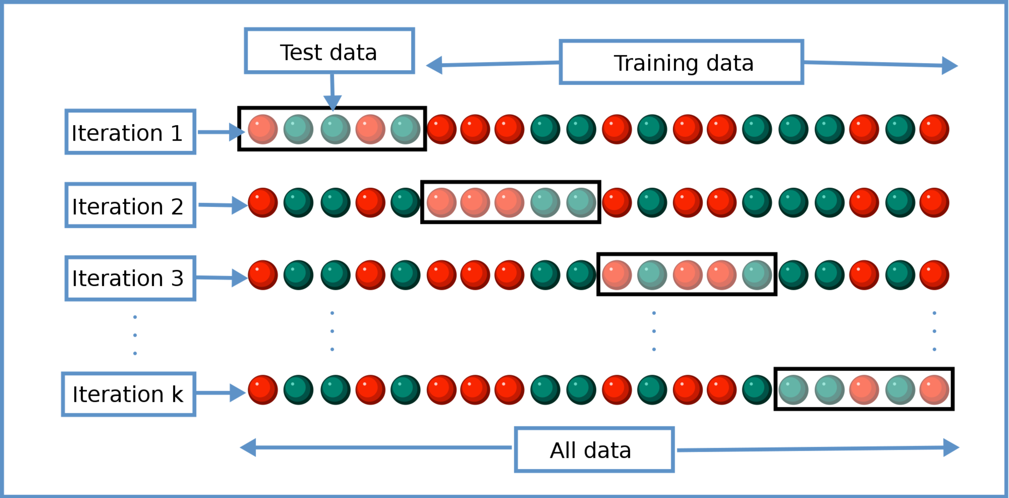
We repeat this process for multiple epochs. For each epoch, repeat the process described above, continuing to train the kdifferent models on the appropriate data and re-testing it on its test fold. In this project, we supply two different averages of the model's accuracy in cross-validation.
Fold Superscore Cross-Validation Accuracy: Suppose we perform k-fold cross validation for e epochs. In this measure of accuracy, for each fold, we select the highest accuracy achieved for the fold across all the e epochs. Then, with those kmaximum accuracies, we compute the average. In doing so, we average the model's best possible performance on each fold, no matter when that maximum occurred in the training/testing process.
Maximum Epoch Cross-Validation Accuracy: This is the widely used measure of cross-validation accuracy. In this metric, we simply average the accuracies of all folds at the end of each epoch. After we've completed all the epochs, we select the epoch that had the highest average across all the folds, and output that average.
Starting with a Basic Model
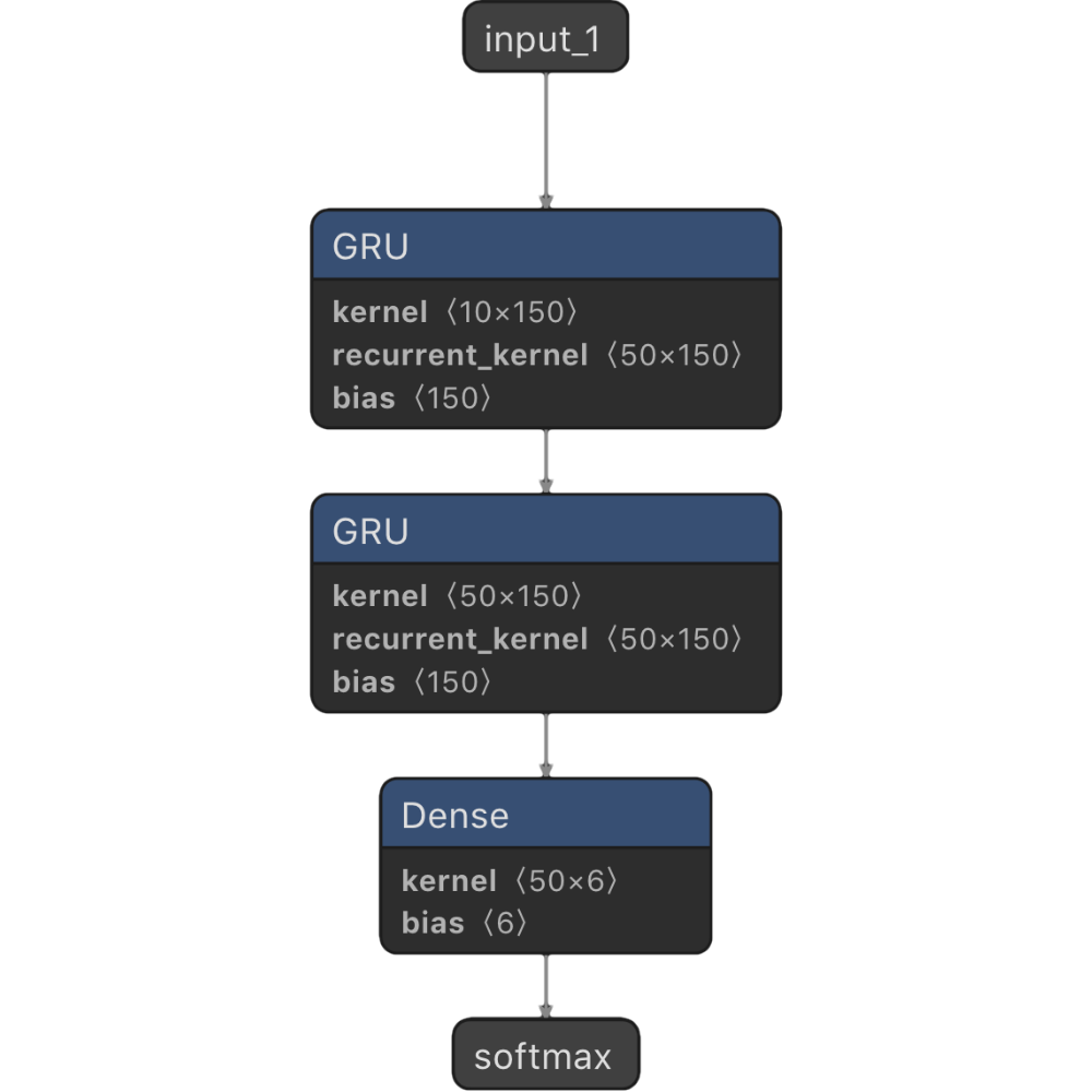
Constructing a Simple GRU Model
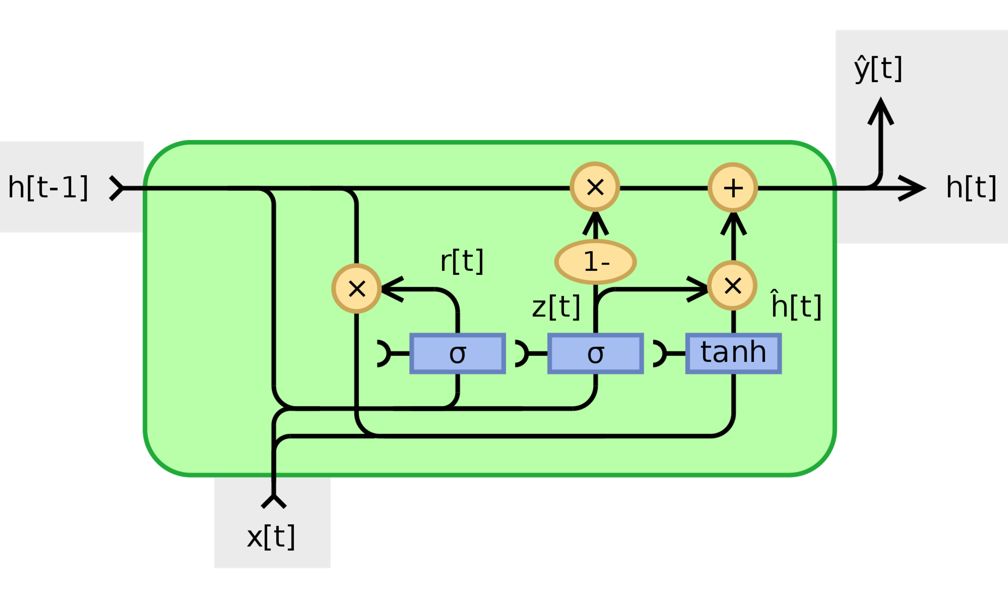
The first model I constructed was a simple GRU model (SimpleGRU). This model consists of an input layer for the current window of MFCC features, plus a variable number of GRU (Gated Recurrent Unit) layers of variable size, and a softmax output layer. GRU layers are a type or recurrent neural network. Recurrent neural networks are useful in temporal sequences of data, because their predictions at a given time step are influenced by the inputs for timesteps in the past.
At a high level, the idea behind the GRU layer(s) is to give the model “memory” such that at a given time step, the current model prediction is dependent upon past inputs. This makes sense intuitively, as a human would rely heavily on memory for accomplishing this task: when determining if the song has changed from verse to chorus, a human would need to remember what the verse sounded like in order to decide that the song presently sounds different and has thus entered a chorus.
If you're curious about how GRUs work, you can read this excellent article.
If you're following along in the code that I wrote, you can instantiate the SimpleGRU model and perform cross-validation using code like below. I wrote all the model classes in a way that was easy for me to tweak parameters and adjust inputs without digging through lines of code to change things, but all of these classes are build atop the Keras open-source neural-network library.
#Instantiate and build the SimpleGRU model

model = SimpleGRU(modelName)
model.build(inputDimension=10,numPerRecurrentLayer=50,
    numRecurrentLayers=2, outputDimension=6)
model.summary()


#Make data generator modules to read in MFCC features from
#"features/mfcc_input_1"

modulesList =[]
mFCCDataGeneratorModule = BasicDataGeneratorModule("features", "mfcc_input_1", outputExtraDim=True)
modulesList.append(mFCCDataGeneratorModule)


#Instantiate a GeneratorLabeler1D to make labels from
#annotations in "annotations"
generatorLabeler = GeneratorLabeler1D("annotations", 22050,
    hop_length)


#Instantiate the data generator with the modules and labeler
modularDataGenerator = ModularDataGenerator("features", "labels",
    modulesList, generatorLabeler, samplesShapeIndex=1,
    outputExtraDim=True)


#Instantiate an evaluator on the data generator
evaluator = ModelEvaluator(modularDataGenerator)


#Actually perform training/12-fold cross-validation for 10 epochs
evaluator.trainWithKFoldEval(model=model, k=12, modelName="SimpleGRU",
    epochs=10, saveBestOnly=False, outputExtraDim=True)
Missing Ingredients?
Unfortunately, this model doesn’t perform very well, as seen above. My conjecture for the poor performance is as follows: The sequence is too long for the recurrent layers to be effective. In the raw MFCC data extracted at hop lengths of 2048 samples on audio with sample rate 22050Hz, a 20-second chorus would produce 20*22050/4096 = ~108 consecutive time steps with the same label. With so many time steps labeled the same, it may be difficult for the GRU units to decide which memories are important to keep to make good predictions, and which can be forgotten. Moreover, a long stretch of data from a chorus may exhaust the recurrent layers' capacity to remember other parts of the song, such as a verse or bridge. In any case, the model is probably being overloaded with information!
Fold Superscore Cross-Validation Accuracy: 49.91%
Maximum Epoch Cross-Validation Accuracy: 46.98%
Unfortunately, this model doesn’t perform very well, as seen above. My conjecture for the poor performance is as follows: The sequence is too long for the recurrent layers to be effective. In the raw MFCC data extracted at hop lengths of 2048 samples on audio with sample rate 22050Hz, a 20-second chorus would produce 20*22050/4096 = ~108 consecutive time steps with the same label. With so many time steps labeled the same, it may be difficult for the GRU units to decide which memories are important to keep to make good predictions, and which can be forgotten. Moreover, a long stretch of data from a chorus may exhaust the recurrent layers' capacity to remember other parts of the song, such as a verse or bridge. In any case, the model is probably being overloaded with information!
Breakthrough 1: Pooling Past Windows
Expanding the Model's View of the Song
As mentioned earlier, my hypothesis regarding the SimpleGRU implies that our model is being required to "remember" too much past data to make a prediction. To fix this, I decided to make a model that "pools" past MFCC frames. So, instead of having a single input layer for the current frame of MFCC, the model might benefit from being fed past frames of MFCC data. This should reduce the model's burden in choosing information to store and forget, and reduce the burden to "remember" past MFCC frames.
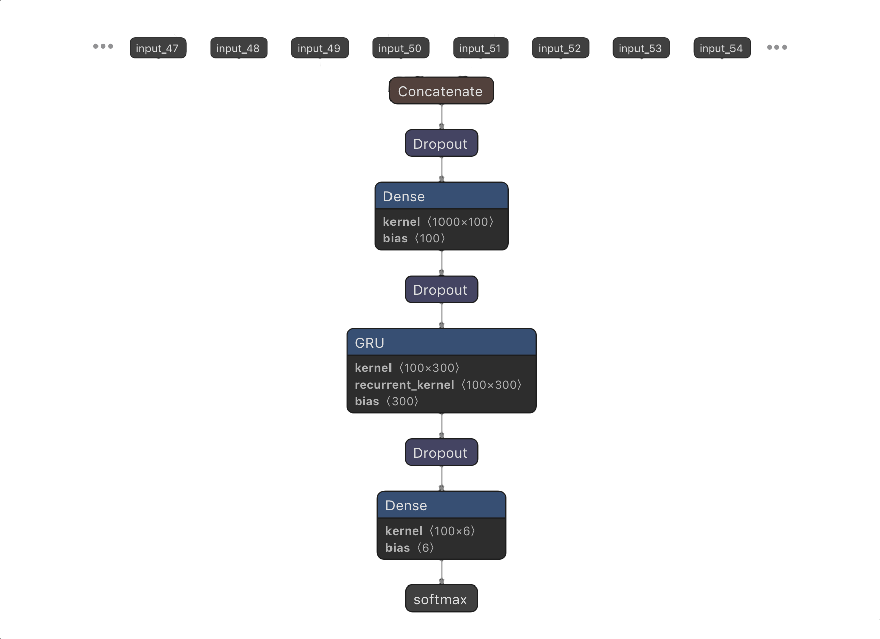
Basic Pooling
In response to this hypothesis, I made the PoolingModelWithDropout model. (NOTE: for those of you with a machine learning background, this has no relation to max pooling) This model (shown above) takes an adjustable number of input layers, each of which takes in a window of MFCC data. For example, Input 0 takes in MFCC data from the current time step (i.e. MFCC from the past 8192 samples if n_fft=8192), input 2 takes in data from the previous time step (i.e. from the window of 4096-12,288 samples before the current sample), and so on. In doing so, the model is allowed to see a limited window of what the song sounded like in the recent past. Note that the dropout layers were added to reduce overfitting, the tendency of the model to fit the training data very well at the expense of accuracy in test data.
Furthermore, the concatenation of all of these input layers was passed through a ReLU layer, which was then connected to the GRU recurrent layers. This ReLU layer was also introduced to combat overfitting, as limiting the size of this layer limits the amount of information that flows to the recurrent layers. In doing so, the recurrent layers are less likely to see small eccentricities in the training data that might allow them to perform well on training data but bad on test data where these eccentricities are not present.
The model was constructed with a dropout rate of 0.45, a pool size of 500 (I.e. at each time step the model will receive the current window of MFCC features plus the last 499 windows), a dense layer of 100 units, and 1 recurrent layer with 100 units.
You can instantiate the PoolingModelWithDropout model and perform cross validation in the code I wrote like so:
#Build the model

model = PoolingModelWithDropout(modelName)
model.build(dropoutRate=0.45, numInputs=500, perInputDimension=n_mfcc,
    numPerRecurrentLayer=100, numRecurrentLayers=1,
    numDenseLayerUnits=100, outputDimension=6, outputExtraDim=True)
model.summary()


#Make data generator modules to read in MFCC features from
#"features/mfcc_input_1"

modulesList =[]
pooledDataGeneratorModule = PooledDataGeneratorModule(poolSize,
    "features", "mfcc_input_1", outputExtraDim=True)
segmentOrderDataGeneratorModule = SegmentOrderDataGeneratorModule(
    "features","segment_order_input_1", outputExtraDim=False)
modulesList.append(pooledDataGeneratorModule)


#Instantiate a GeneratorLabeler1D to make labels from
#annotations in "annotations"

generatorLabeler = GeneratorLabeler1D("annotations", 22050, hop_length)


#Instantiate an evaluator on the data generator

modularDataGenerator = ModularDataGenerator("features", "labels",
    modulesList, generatorLabeler,samplesShapeIndex=1, outputExtraDim=True)


#Actually perform training/12-fold cross-validation for 10 epochs

evaluator = ModelEvaluator(modularDataGenerator)
evaluator.trainWithKFoldEval(model=model, k=12, modelName=modelName,
    epochs=10, saveBestOnly=False, outputExtraDim=True)
Fold Superscore Cross-Validation Accuracy: 61.37%
Maximum Epoch Cross-Validation Accuracy: 56.01%
As seen above, this model achieved markedly better performance than SimpleGRU. Unfortunately, this model took significantly longer to train and evaluate than SimpleGRU, which is expected from the significant increase in complexity.
Faded Pooling
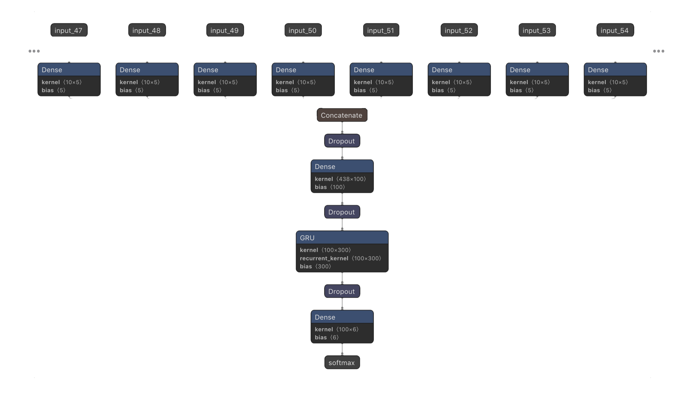
To further reduce overfitting, I added ReLU layers after each of the input layers, each of varying sizes. Specifically, the first input layer (the one taking in the current frame of MFCC data) had a 5-unit layer, and the last input layer (taking in MFCC data from the distant past) was given a 1-unit layer. The number of units per layer for the inputs in-between the first layer with 5 units and the last layer with 1 unit was interpolated using logarithmic decay (so that input layers with MFCC windows further in the past had ReLU layers with less units than input layers with recent or current MFCC windows). My goal in adding these ReLU layers was to limit the amount of information coming from input layers, especially the information from the distant past. By forcing information from input MFCC frames from the distant past to go through small layers, the later layers in the model (such as the GRUs) have a simplified view of what the song sounded like in the distant past.
You can instantiate the FadingPoolingModelWithDropout model and perform cross-validation like this:
#Build the model

model = FadingPoolingModelWithDropout(modelName)
model.build(dropoutRate=0.45, numInputs=500, perInputDimension=n_mfcc,
    numPerRecurrentLayer=100, numRecurrentLayers=1,
    numDenseLayerUnits=100, outputDimension=6,
    fadingMaxUnits=5, outputExtraDim=True)
model.summary()


#Make data generator modules to read in MFCC features from
//"features/mfcc_input_1"

modulesList =[]
pooledDataGeneratorModule = PooledDataGeneratorModule(poolSize,
    "features", "mfcc_input_1", outputExtraDim=True)
segmentOrderDataGeneratorModule = SegmentOrderDataGeneratorModule(
    "features","segment_order_input_1", outputExtraDim=False)
modulesList.append(pooledDataGeneratorModule)


#Instantiate a GeneratorLabeler1D to make labels from
#annotations in "annotations"

generatorLabeler = GeneratorLabeler1D("annotations", 22050, hop_length)


#Instantiate an evaluator on the data generator

modularDataGenerator = ModularDataGenerator("features", "labels",
    modulesList, generatorLabeler,samplesShapeIndex=1, outputExtraDim=True)


#Actually perform training/12-fold cross-validation for 10 epochs

evaluator = ModelEvaluator(modularDataGenerator)
evaluator.trainWithKFoldEval(model=model, k=12, modelName=modelName,
    epochs=10, saveBestOnly=False, outputExtraDim=True)
Fold Superscore Cross-Validation Accuracy: 62.74%
Maximum Epoch Cross-Validation Accuracy: 57.42%
This modification to the pooling architecture produces small increases in accuracy compared to PoolingModelWithDropout's accuracy, although I'm not sure if these increases are statistically significant.
However, these models seem very bloated and possibly still overloaded with information. They are still being asked to classify every 4096 samples, which corresponds to approximately every 1/5 of a second in our 22,050Hz audio. That seems like a lot of redundant information and classifications!
Breakthrough 2: Convolution Over MFCC Windows
The second breakthrough occurred by restructuring the model to take pools of past MFCC frames as 2D inputs, and apply convolutional neural networks on each of them.
Convolutional Neural Networks and MFCC Pools
As I learned in 6.036 at MIT last fall, convolutional neural networks are useful for solving problems where the patterns in the input exhibit spatial locality and translation invariance. A commonly used example in images is finding patterns of pixels that correspond to a cat: spatial locality means that all of the pixels that make up the cat in the image will be near each other, and translational invariance means that certain pixel patterns characterize a cat no matter where they occur in an image.
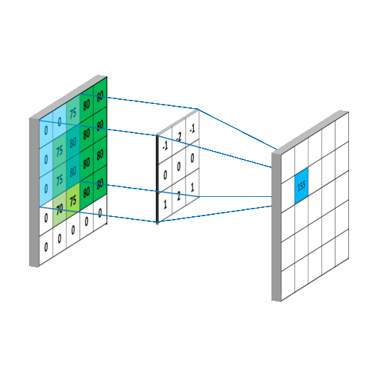
How might this apply to pools of MFCC features extracted from audio? Consider a pool of extracted MFCC features, where the X dimension is a row of extracted MFCC coefficients for a given window, and the Y dimension are the different rows of MFCC windows. Suppose we are interested in patterns of MFCC features that correspond to the sound of cymbals. These patterns exhibit spatial locality, because the sound of cymbal will be distributed over consecutive MFCC windows, and they exhibit translational invariance, because certain MFCC patterns can occur at the beginning (recent) part of the pool or the end part (less recent) part of the pool.
If you're interested in how convolutional neural networks actually work, take a look at this article!
Faded2DConv: Network Architecture
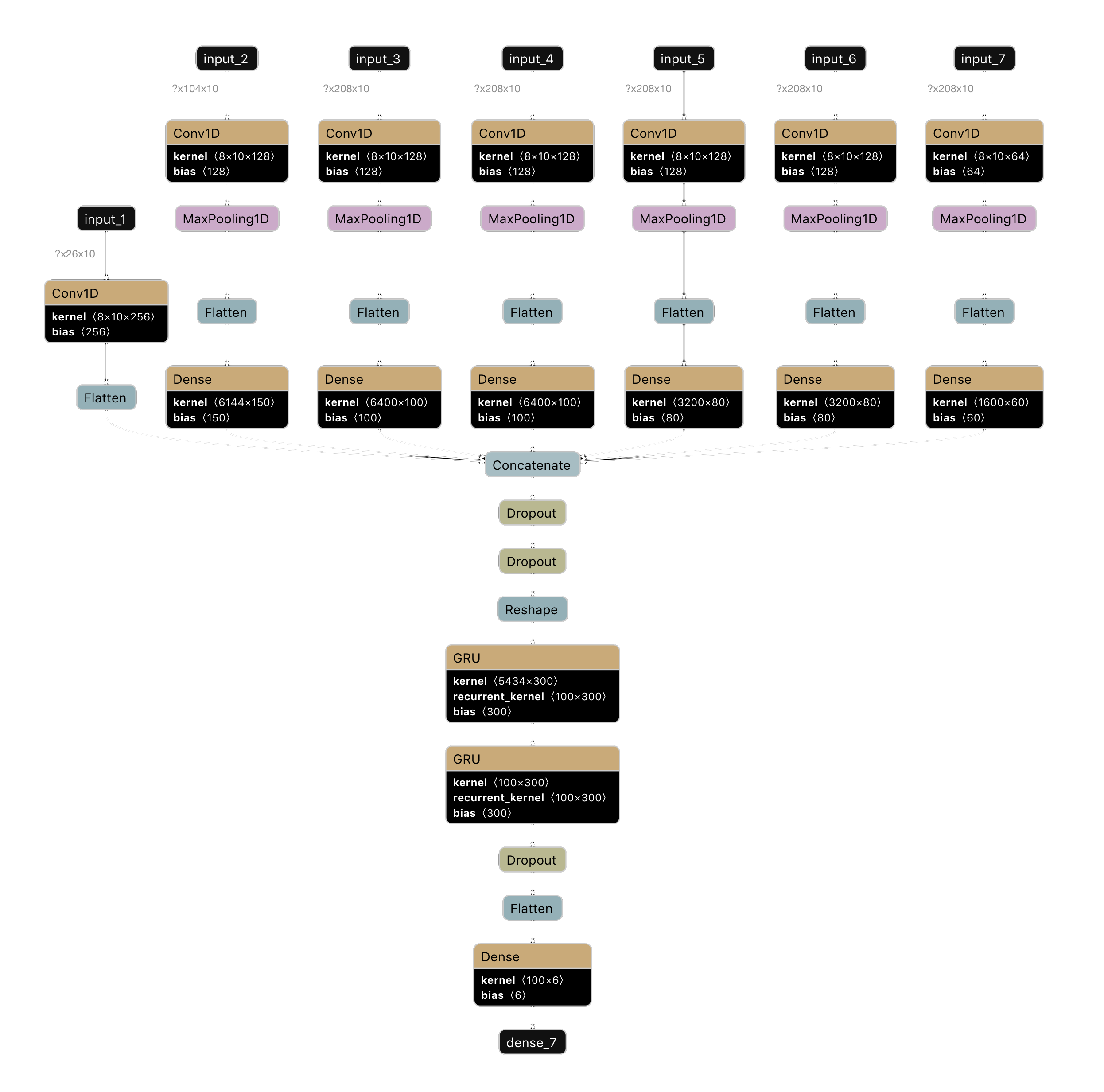
As mentioned before, the breakthrough with this model is structuring the pools of past MFCC windows as 2D inputs. In the previous models, each input layer would take 1-dimension input – a single row of MFCC coefficients for a single MFCC window. In this model, a single input layer takes in multiple MFCC windows, which are concatenated together in 2D input. For instance, the first input layer in this model takes in a pool of 26 MFCC windows – i.e. it is a 26 x 10 array, where each of the 26 rows contains 10 MFCC coefficients, with row 0 being the current MFCC window's coefficients, and row 26 being the MFCC coefficients for the window corresponding to samples (26*4096) to (26*4096+8192).
By structuring the pools in two dimensions, we can perform convolutional neural networks over them. Specifically, the Faded2DConv uses Keras's Conv1D layer.
The Faded2DConv model that I used included 6 different 2D pools. The first 2D pool included MFCC windows 0-26, the second included windows 26-130, the third included windows 130-338, the fourth included windows 338-546, the fifth included windows 546-754, and the sixth included windows 754-962, and the 7th included windows 962-1,170. In terms of seconds, these MFCC pools span 1170*4096/22050 = ~217 seconds. That is, our model gets to see the past ~217 seconds of the song! Note that for timesteps before ~217 seconds, the pools that stretch backwards beyond the MFCC window are zero-padded.
For each of the 2D input pools, there is a convolutional layer. The first had 256 filters, the second through sixth had 128 filters, and the 7th had 64 filters. The fewer the filters, the less information that can be extracted from the input. This is precisely the reason I decreased the number of filters for pools with MFCC windows from the distant past – the model should have a less detailed view of the previous parts of the song than the more recent parts of the song.
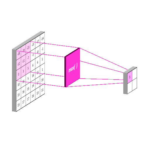
Additionally, the second had a max pooling layer with kernel size 2, the third and fourth had a max pooling layer with kernel size 4, and the fifth through 7th had a max pooling layer with kernel size 8. Max pooling helps with dimensionality reduction. A 1D max pooling layer 2 will have output half the size of its input. Intuitively, a max pooling layer reduces the amount of information because it reduces the amount of detail when transforming its input to its output (as a 5 number output will surely have less capacity to store information than the original 10 number input). Again, this is consistent with the idea that the model should see less detail from previous parts of the song.
Next, the output of the max pooling layers for inputs 2-7 were passed through dense layers of sizes 150,100,100,80,80, and 60, respectively.
The output of these layers plus the output of the convolutional layer for input layer 1 (i.e MFCC windows 0 through 26) was then concatenated and passed through two dropout layers (of dropout rates 0.35 and 0.5).
Next are two recurrent GRU layers of size 100, each with recurrent dropout=0.5.
Finally, the output of the second GRU layer was passed through another dropout layer (with dropout rate=0.5) onto a final 6 unit softmax layer for output.
If you're interested in trying out Faded2DConv on your own, you can use my code as follows:
#Build the model

model = Faded2DConvModel(modelName)
model.build(numClasses=numSegmentTypes, inputShapeList=[(26,10),(104,10),(208,10),(208,10),(208,10),(208,10),(208,10)],
                inputConvFilterNumList=[256, 128, 128, 128, 128, 128, 64],
                inputConvKernelSizeList=[8,8,8,8,8,8,8], convMaxPoolSizeList=[None, 2, 4, 4, 8, 8, 8],
                convDenseSizeList=[None,150,100,100,80,80,60],
                postConvDropout=0.35, preRNNDropout=0.5, rNNUnitsList=[100,100], rnnDropoutList=[0.5,0.5],
                postRNNDropout=0.5)
model.summary()


#Make modules to extract the pools of data

modulesList =[]
chunkedMFCCDataGeneratorModuleNear = ChunkedMFCCDataGeneratorModule("features", "mfcc_input_1", 26, 13)
chunkedMFCCDataGeneratorModuleMid = ChunkedMFCCDataGeneratorModule("features", "mfcc_input_1", 104, 13)
chunkedMFCCDataGeneratorModuleFar = ChunkedMFCCDataGeneratorModule("features", "mfcc_input_1", 208, 13)

delayed2DDataGeneratorModuleMid = Delayed2DDataGeneratorModule(chunkedMFCCDataGeneratorModuleMid, 2)
delayed2DDataGeneratorModuleFar = Delayed2DDataGeneratorModule(chunkedMFCCDataGeneratorModuleFar, 10)
delayed2DDataGeneratorModuleVeryFar = Delayed2DDataGeneratorModule(chunkedMFCCDataGeneratorModuleFar, 26)
delayed2DDataGeneratorModuleVeryVeryFar = Delayed2DDataGeneratorModule(chunkedMFCCDataGeneratorModuleFar, 42)
delayed2DDataGeneratorModuleSuperFar = Delayed2DDataGeneratorModule(chunkedMFCCDataGeneratorModuleFar, 58)
delayed2DDataGeneratorModuleSuperDuperFar = Delayed2DDataGeneratorModule(chunkedMFCCDataGeneratorModuleFar, 74)

modulesList.append(chunkedMFCCDataGeneratorModuleNear)
modulesList.append(delayed2DDataGeneratorModuleMid)
modulesList.append(delayed2DDataGeneratorModuleFar)
modulesList.append(delayed2DDataGeneratorModuleVeryFar)
modulesList.append(delayed2DDataGeneratorModuleVeryVeryFar)
modulesList.append(delayed2DDataGeneratorModuleSuperFar)
modulesList.append(delayed2DDataGeneratorModuleSuperDuperFar)


#Instantiate a GeneratorLabeler2D to make labels from
#annotations in "annotations"

generatorLabeler = GeneratorLabeler2D("annotations", 22050, hop_length, 13)


#Instantiate an evaluator on the data generator

modularDataGenerator = ModularDataGenerator("features", "labels", modulesList, generatorLabeler, samplesShapeIndex=0, outputExtraDim=True)
evaluator = ModelEvaluator(modularDataGenerator)


#Actually perform training/24-fold cross-validation for 10 epochs

evaluator = ModelEvaluator(modularDataGenerator)
evaluator.trainWithKFoldEval(model=model, k=24, modelName=modelName, epochs=10, saveBestOnly=False, outputExtraDim=True)
Performance
Whew! That was a lot! But it was worth it! Take a look:
Fold Superscore Cross-Validation Accuracy: 70.19%
Maximum Epoch Cross-Validation Accuracy: 62.87%
This is especially impressive performance for our model! It means that for a song that the model has never heard before, the model architecture specified by Faded2DConv is, for some amount of training, capable of labeling 70% of the song correctly.
Keep in mind, these are songs for which the model has never been given labels before. The model architecture is capable of being trained to produce the correct song segment type 7 out of 10 times in a new song!
Discussion
Although the cross validation statistics are exciting, the final Faded2DConv model was extremely prone to overfitting, even with the extreme amount of dropout added! At just epoch 2, with dropout on, the most folds had models that were producing training accuracies in the 50% range. The model was trained for only 15 epochs, and even with dropout on, the some model folds approached mid 80% training accuracies around epoch 11.
The takeaway about this is that the model either needs more structural changes to help it avoid overfitting (perhaps even more dropout, increase in max pool kernel size, or reduction in number of filters, dense layer sizes, etc), and/or the model needs more training data. 24 songs to train upon is not a lot of training data. It is possible that this model will generalize more and avoid overfitting when supplied with more training data (I love Waymaker, but for the sake of our model, perhaps worship pastors should sing some other songs!).
Finally, although cross-validation is great for determining the potential performance of this model structure, it is not a direct measure of accuracy on real-world test data. Unfortunately, at the moment I don't really have enough data to train the model more and create a test dataset (I should probably study for my midterms right now instead of scouring my church's YouTube channel for services with different songs).
Conclusion: To Be Continued
In conclusion, there is still work to be done to understand how well MusicSegmentationML performs in the real world and how it can be improved. However, the results of Faded2DConv are impressive – I'm not sure I would be able to execute the correct cues 70% of the time for a song I have never heard before!
As discussed, further evaluation (with a larger set of training and dedicated test data) of the the Faded2DConv is necessary to evaluate its true real-world performance. During my spring break, I intend to revisit this project, adding more labeled audio and possibly tweaking the model's structure. I spoke with my friends Noah and Nimit about this project, specifically about the possibility of adding an attention layer to help the model decide which stored memories in the recurrent layers are important for making predictions at a given timestep, but I need to understand how this mechanism works better before I use it in practice.
I also hope to one day use this model for live inference – i.e. allow the model to make predictions on features extracted from a live audio stream. Perhaps I might even work on an interface with the lighting console at my church so that the model can dictate which lighting cue is active based on its predictions during a worship rehearsal (or actual worship service, contingent on how much M trusts the neural network).
I would also really appreciate any feedback you may have on this project or article – including questions, comments, criticisms, corrections, or suggestions! You can send me an email at me[at]nathancontreras(dot)com. If you have an idea for a new model architecture, different features, or want to help with data collection, let me know!
-Nathan
